안녕하세요 '코딩 오페라'블로그를 운영하고 있는 저는 'Conducter'입니다.
오늘 알아볼 내용은 Support Vector Machine(SVM)입니다.
서포트 벡터 머신(support vector machine, SVM) : 기계 학습의 분야 중 하나로 패턴 인식, 자료 분석을 위한 지도 학습 모델이며, 주로 분류와 회귀 분석을 위해 사용한다.

위의 그림과 같이 SVM은 데이터에서 그룹을 분류하는 알고리즘 중 하나입니다. 그룹에서 중 상대 그룹과 가장 가까운 데이터끼리의 거리를 Margin이라 하고 이 Margin값이 가장 크도록 그룹을 분류하는 방식입니다. 여기에 대한 수학적 해석은 다음번에 다루도록 하고 오늘은 SVM응용에 대해 알아보도록 하겠습니다.
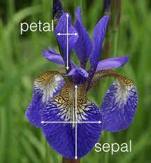
오늘 다룰 내용은 'iris'즉 붓꽃을 분류하는 예시 입니다. iris는 위의 사진처럼 petal과 sepal이라는 두 부분으로 나뉘는 데 이 부분의 길이와 너비에 따라 iris의 종류가 나뉩니다.
먼저 아래와 같이 기본 라이브러리들을 불러줍니다. 여기서 sklearn의 내장되어 있는 iris data를 가져옵니다.
import pandas as pd
import numpy as np
import matplotlib.pyplot as plt
from sklearn.linear_model import LinearRegression
#머신러닝 분석에 유용한 라이브러리
from sklearn.datasets import load_iris
iris = load_iris()
# sklean에서 iris데이터를 가져온다.
from sklearn.model_selection import train_test_split
from sklearn.svm import SVC
iris 데이터의 feature를 알아보면 다음과 같이 'sepal length', 'sepal width', 'petal length', 'petal width' 이렇게 4가지가 있는 것을 확인할 수 있습니다.
iris.feature_names['sepal length (cm)',
'sepal width (cm)',
'petal length (cm)',
'petal width (cm)']
pandas의 pd.DataFrame 함수를 이용해 데이터 프레임을 만들어주고 'target' feature를 추가해줍니다.
df = pd.DataFrame(iris.data, columns=iris.feature_names)
# 데이터 프레임을 만들어줌

df['target'] = iris.target
# 'target' feature를 만들어줌
데이터 프레임을 봐주면 아래와 같이 'target'이 추가된 모습을 확인 할 수 있습니다.

iris target이름을 확인해 줍니다. 여기서는 'setosa'=0, 'versicolor'=1, 'virginica'=2입니다.
iris.target_names
# 'setosa'=0, 'versicolor'=1, 'virginica'=2
array(['setosa', 'versicolor', 'virginica'], dtype='<U10')
apply함수를 이용해 각 target의 꽃 이름을 추가해 줍니다.
df['flower_name'] = df.target.apply(lambda x: iris.target_names[x])
# iris의 target_names을 apply하여 이름을 나타내어줌
각 꽃의 종류별로 데이터 프레임을 분류해줍니다.
df0 = df[df.target==0]
df1 = df[df.target==1]
df2 = df[df.target==2]
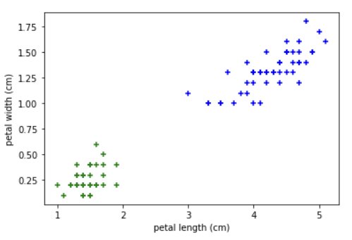
sepal과 petal에 대해 각각 그래프를 그려주면 아래와 같습니다.
plt.scatter(df0['sepal length (cm)'], df0['sepal width (cm)'], color = 'green', marker = '+')
plt.scatter(df1['sepal length (cm)'], df1['sepal width (cm)'], color = 'blue', marker = '+')
plt.xlabel('sepal length (cm)')
plt.ylabel('sepal width (cm)')
plt.scatter(df0['petal length (cm)'], df0['petal width (cm)'], color = 'green', marker = '+')
plt.scatter(df1['petal length (cm)'], df1['petal width (cm)'], color = 'blue', marker = '+')
plt.xlabel('petal length (cm)')
plt.ylabel('petal width (cm)')

X와 y데이터를 지정해줍니다.
X = df.drop(['target', 'flower_name'], axis = 'columns')
y = df.target
train_test_split함수를 통해 train data와 test data를 분리해줍니다. 여기에서는 test data비율을 20%로 했습니다.
X_train, X_test, y_train, y_test = train_test_split(X, y, test_size=0.2)
위에서 불러온 SVC라이브러리를 통해 SVM model을 만들어줍니다. 여기서 C값이 클수록 오류를 허용하지 않는 hard margin, C값이 작을수록 오류를 허용하는 soft margin입니다.
model = SVC(C=10)
# C값이 클수록 하드마진(오류 허용 안 함), 작을수록 소프트마진(오류를 허용함)이다.
# shift tab으로 SVC확인!(여러 파라미터들이 있다.)
train data를 이용해 model을 fit 해준 다음, test data로 model의 score을 계산해주면 약 0.967 정도가 나와서 상당히 잘 학습한 것을 알 수 있습니다.
model.fit(X_train, y_train)

model.score(X_test, y_test)
오늘은 Support Vector Machine(SVM)에 대해 알아보았습니다. 도움이 되셨나요? 만약 되셨다면 구독 및 좋아요로 표현해 주시면 정말 많은 힘이 됩니다. 궁금한 사항이 있으시면 댓글 남겨주시면 감사하겠습니다. 저는 '코딩 오페라'의 'Conductor'였습니다. 감사합니다.
<출처 및 참고 : 위키백과, code basics>
'머신러닝' 카테고리의 다른 글
| 나이브 베이즈 분류 알고리즘(Naive Bayes Classifier Algorithm), 타이타닉 생존자 예측 (0) | 2022.01.27 |
|---|---|
| K-평균 알고리즘(K-means clustering algorithm) (0) | 2022.01.20 |
| 로지스틱 회귀(Logistic Regression) (2) | 2022.01.12 |
| 학습 데이터와 훈련 데이터(Training Data and Testing Data) (0) | 2022.01.12 |
| 선형 회귀 모델의 수학적 해석(Gradient Descent and Cost Function) (0) | 2022.01.11 |